Estimating the Best Price Elasticity Function

by Roshni Mohandas

After we have extracted the data which contains demand at various price points, we will have to estimate price elasticity functions. The reason is that the price elasticity function will give the best representation of how consumers respond to price and what will be the demand of the product

We will be doing this for each product at a store level, we can also go about doing this for different customer segments for better accuracy (Check out the blog on Challenges of Pricing). The price demand function will also be different for different stores selling the same product due to many factors such as perceived value, location, etc.

In a textbook definition, the price function faced by different sellers is linear at the market price. If a seller sells an item at discount, the demand increases, and when the seller increases the price, demand falls. In a perfectly competitive market, the seller has no pricing decisions - the price is decided by the market.

We will discuss the most common price elasticity functions below:

Normal Distribution

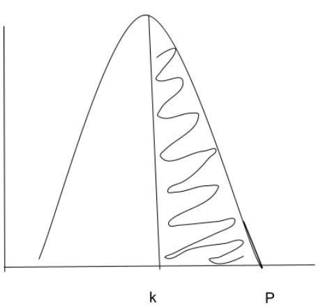
In the above graph, if k and P are Rs.20 and Rs.50, then we can say almost half of the population has a willingness to pay equal to 30 rupees

Since the function is a bell curve or normal distribution, it is a good assumption that most of the buyers would fall around the mean which would be Rs.20 +/- standard deviation. The customers who are falling on the right are high-end customers and on the left are low-end.

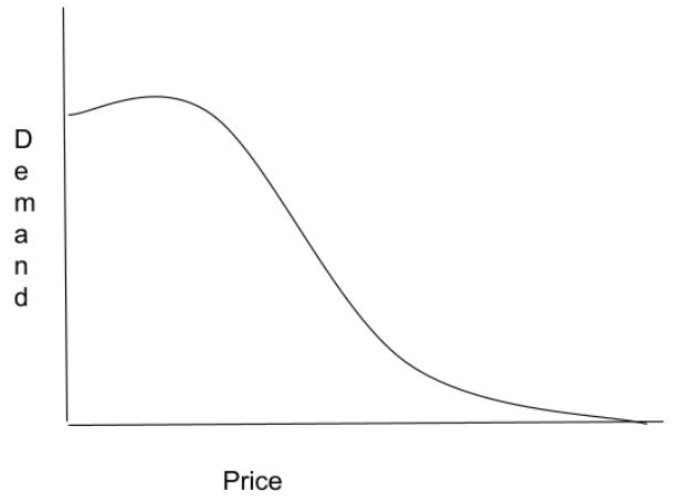
The price response function derived from the bell curve has a reverse S shape as shown below: 

For the S curve, returns are drastically reduced when making large price decreases. Also, the curve is flat for high prices.

Linear Price Elasticity Function

The linear price elasticity function is nothing but the familiar equation which we use in linear regression

Price Function(d(p))  = Intercept + slope * independent_variable

This function is used commonly as its is easy to estimate.

Constant Elasticity Price Functions

In such cases, the elasticity will be the same at all prices. This will be an exponential function.

d(p) = Cpε

In the above equation, C and ε are  found by fitting equation to the price/demand data

Power Price Elasticity Function

This function has a reverse S shape

d(p) = α * D/(pβ+α)

In the above equation D , α and β are parameter values estimated by fitting the equation to the price demand data. Higher value of β represents more sensitive markets. As β grows larger, the market reaches the perfectly competitive price elasticity.

Logit Price Elasticity Function

Another common price response curve that has a reverse S shape functional form is the logit function

dp = C*ea+b*p/1+ea+b*p

Here C, a, b are parameters that are estimated by fitting the equation

Summary:

Loved the blog? Do check out another awesome blog by Roshni Mohandas on Pricing Analytics Process.

Struggling to price your products? Book a demo with our pricing experts now!!